Using agent based modeling to predict Digital euro adoption

A technical companion to an upcoming OMFIF commentary article

This post explains my Digital Euro Adoption code repository, which uses agent based modeling and machine learning to predict how three product decisions could affect adoption of the Digital Euro:

• How long can sign-up take before people lose interest?

• Does paying in a shop need to be as quick as using a physical card?

• How fast does a person-to-person (P2P) payment need to feel?

This post explains how the model works and the key assumptions behind it, while an upcoming post from OMFIF will discuss business and policy implications. I’ll link to that article when it becomes available.

At a high level, I modeled 100,000 simulated buyers using a combination of supervised and reinforcement learning. Each buyer has their own weights and learns whether a new payment method is worth signing up for. Buyers who sign up also learn when to use it instead of cash, a card or a bank transfer.

I start with payment times based on Sweden’s Swish system, then change one Digital Euro assumption at a time and compare the results. As such, this is a scenario model, not a forecast of the Digital Euro’s actual future market share.

Why start with Swish?

Swish is a useful starting point because it is a digital payment method with a similar range of uses. It first became popular as an easy way to send money to another person and later expanded into online and shop payments.

Sweden also publishes data that is useful for creating a reinforcement machine learning model. In particular, the Riksbank measured how long it takes people to complete a transaction using cash, cards and Swish while in-store and online.

And of course, Sweden is in Europe and is part of the European Union. This makes me believe that studying the roll out of a new digital payments system there (even if it is a private solution) is probably more relevant than studying systems like Brazil’s Pix or India’s UPI. This is not to say that Sweden can be thought of as a miniature EU - far from it. However, I believe the political and payments systems landscape that Sweden shares with the rest of the EU makes Swish a useful, if imperfect, comparison.

With all that being said, I use Swish as a sense check and as a source of real payment times, and do not assume that the Digital Euro will follow the same adoption path.

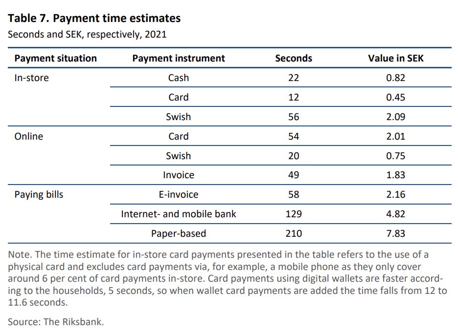
The shop and online times come from Table 7 (below) of the Riksbank’s 2023 Cost of payments in Sweden study. The P2P times and occasional delays are my own assumptions because the table does not include them. We will discuss those assumptions later.

How the model works

Each agent is one buyer with two small neural networks. They start with different random weights. One network estimates how likely the buyer is to sign up. The other scores the payment methods available for each transaction. The code is in BuyerAdoptionRules, BuyerPaymentRules and the shared BuyerNetworks class.

The full model has 100,000 buyers. Every buyer has their own network weights instead of using one network shared by the whole population. PyTorch keeps a separate set of weights for each buyer in the same tensor, then calculates them together with torch.einsum. Both networks have two hidden layers, 32 values in each layer and ReLU activation. The calculation is in BuyerNetworks.apply_hidden_layers.

Each training batch contains 50 payments per buyer (roughly the number of financial transactions an EU citizen completes in a month). The input tensor has one dimension for payments, one for buyers and one for seven input values. The first four inputs show which payment methods are available. The final three show whether the payment is P2P, retail or online. The networks do not see how long each method takes. Payment time is only used as feedback during training.

Main settings

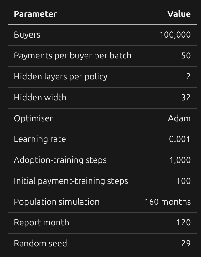
These values are set in consts.py. The model looks for CUDA first and uses 32-bit floating-point numbers.

How payments are created

Each batch represents four weeks. The code chooses a channel for every payment using these fixed probabilities. It also removes methods that cannot be used in that channel.

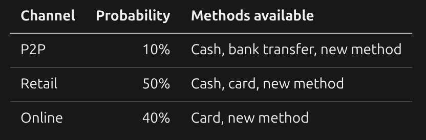
PaymentAdoptionModel._make_sample_payments creates the payments. It chooses the channel, merchant, acceptance and available methods. Five per cent of the 1,000 retail merchants are cash-only for the whole simulation. For the other merchants, the code makes a new acceptance draw for each payment using that month’s acceptance rate.

The formula below calculates the time for buyer b to make payment t with method m. The symbol c is the payment channel. d is the final payment time, while d̄ is the normal time for that method and channel. q is the buyer’s fixed time multiplier for that method. e is the length of a possible extra delay, and z is either zero or one depending on whether that delay happens.

\(d_{btm}=\bar d_{c_t m}q_{bm}+z_{btm}e_{c_t m}q_{bm}\)

The first term is the normal payment time adjusted for the buyer. The second adds the extra delay when z equals one. _realized_payment_durations_for contains the code.

The code draws a separate time multiplier for every buyer and payment method, limited to between two-thirds and 1.5. This lets a buyer be quicker than average with one method and slower than average with another. A separate multiplier changes that buyer’s sign-up time. The draw is in _make_buyer_time_multipliers.

How buyers learn to sign up

For each training batch, the code works out how much time a buyer could save by owning the new method. It finds the quickest available option for every payment, first without the new method and then with it. The calculation is:

\(S_b = \frac{H}{W}\sum_t\left( \min_{m\in A_{bt}^{0}} d_{btm} - \min_{m\in A_{bt}^{1}} d_{btm} \right)\)

In the equation, b identifies the buyer, t the payment and m the method. The two A terms are the methods available without and with the new method. Both H and W are four weeks in these runs. The code then compares the saved time with that buyer's sign-up time:

\(y_b=\mathbf{1}[S_b>o_b]\)

This produces the yes or no answer used to train the network. Buyers do not directly follow this formula when they decide whether to sign up. Their neural networks learn to approximate it from many batches using binary cross-entropy. A sigmoid turns the network's score into a probability, and the buyer makes a random draw using that probability. Once a buyer signs up, they keep the method. The training target is in _adoption_training_loss, and the sign-up draw is in BuyerAdoptionRules.sample_adoption_decisions.

How buyers learn to pay

The payment network gives each method a score. The code removes methods that cannot be used, turns the remaining scores into probabilities and samples one according to those probabilities. There is no hard-coded rule telling buyers to use a particular method in a particular channel. This choice happens in BuyerPaymentRules.sample_payment_methods.

The payment-training loss is:

\(L_b=\sum_t\log\pi_b(a_{bt}\mid x_{bt})d_{bt,a_{bt}}\)

In this equation, a is the chosen payment method, x is the payment input, π is the buyer's payment policy and d is the time taken. This is a simple policy-gradient loss. Longer payments push down the chance of making the same choice again in a similar situation. Payment times are detached from the gradient, so training changes the network rather than the generated times. The code is in _payment_training_loss.

How training works

PaymentAdoptionModel._learn_decision_rules runs 1,000 training steps. Each buyer gets random acceptance rates for P2P, retail and online payments. Ten per cent of the examples use zero acceptance and another 10% use full acceptance. This makes sure the sign-up network sees both extremes.

During the first 100 steps, the payment network learns from payment times. An extra loss keeps its starting chance of choosing the new method close to zero because nobody owns it yet. The sign-up network trains for all 1,000 steps. After step 100, the payment network pauses until the monthly simulation begins. The two networks remain separate: the sign-up network does not copy or inspect the payment network’s weights.

PaymentAdoptionModel._simulate_months then resets ownership to zero and follows the same buyers for 160 months. The sign-up network stops learning, but the payment network updates once each month. P2P acceptance equals the share of buyers who owned the method at the start of that month. Retail and online acceptance rise at a steady rate from zero to 70% over 60 months. The reports use month 120.

Main assumptions

All settings are in consts.py. These are the main assumptions to keep in mind:

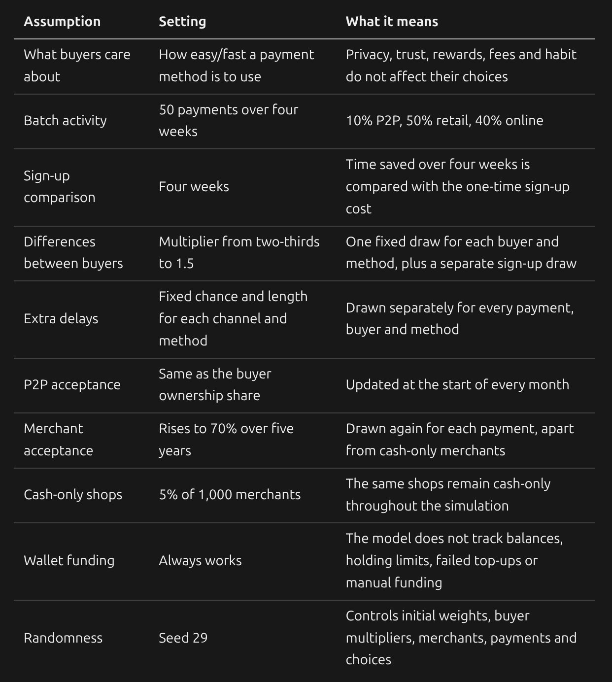
The normal retail and online times for cash, cards and Swish come from the Riksbank table above. The P2P times, chances of extra delays, lengths of those delays and Digital Euro scenarios are my assumptions. The app P2P estimates come from timing myself completing transactions in certain situations. I am probably more technically competent / faster on my phone than the average person, and so added a few seconds / rounded to the nearest 30 seconds to hopefully make things more applicable to a general audience.

The fixed seed makes runs easier to repeat in the same software and hardware setup. Different PyTorch, CUDA or GPU versions may still give slightly different results.

The model also leaves out demographics, geography, payment value, merchant strategy, network capacity, settlement time, privacy, fraud, rewards, fees and legal rules. The Swish run is a basic sense check. I do not fit the model to real Swish adoption data. The Digital Euro runs compare scenarios; they do not forecast future market share.

Scenarios and charts

generate_reports.py lists the settings for every comparison. If the same scenario appears in more than one comparison, the code only runs it once. scenario_results.csv stores the inputs and month-120 results. Quick and full runs write to the same files.

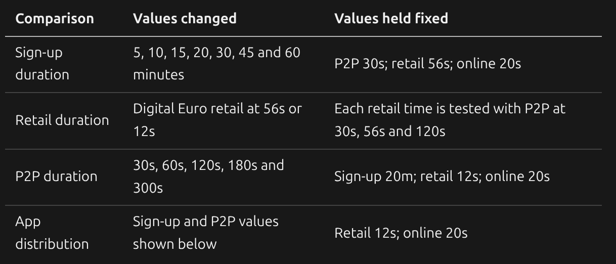
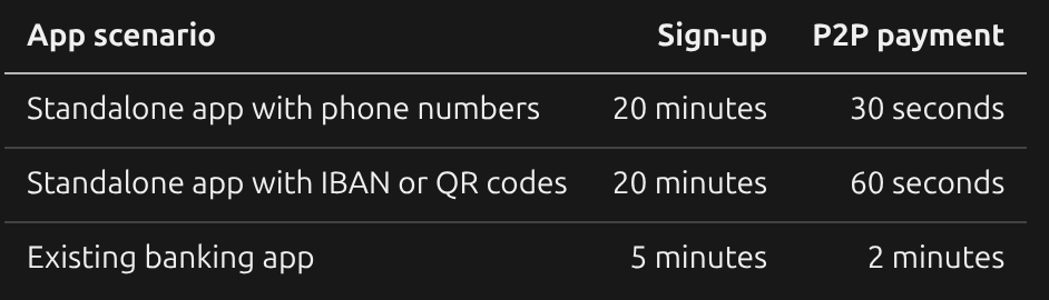
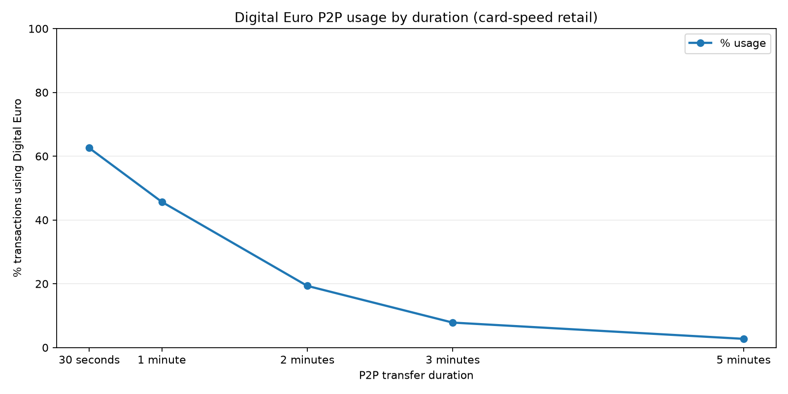
The charts are below. What they mean for policy is discussed in the OMFIF article.

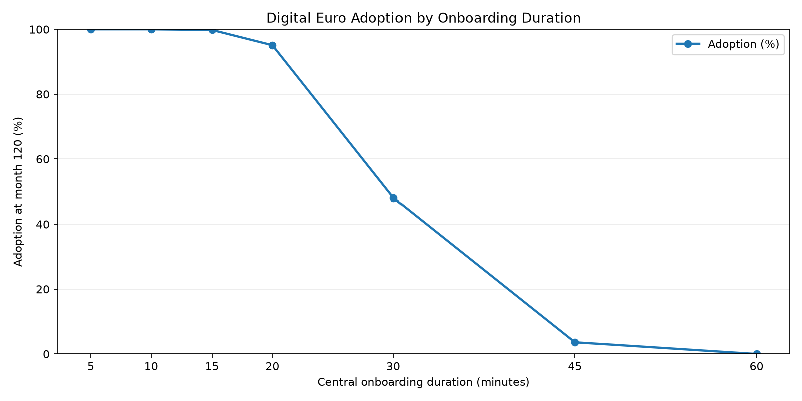
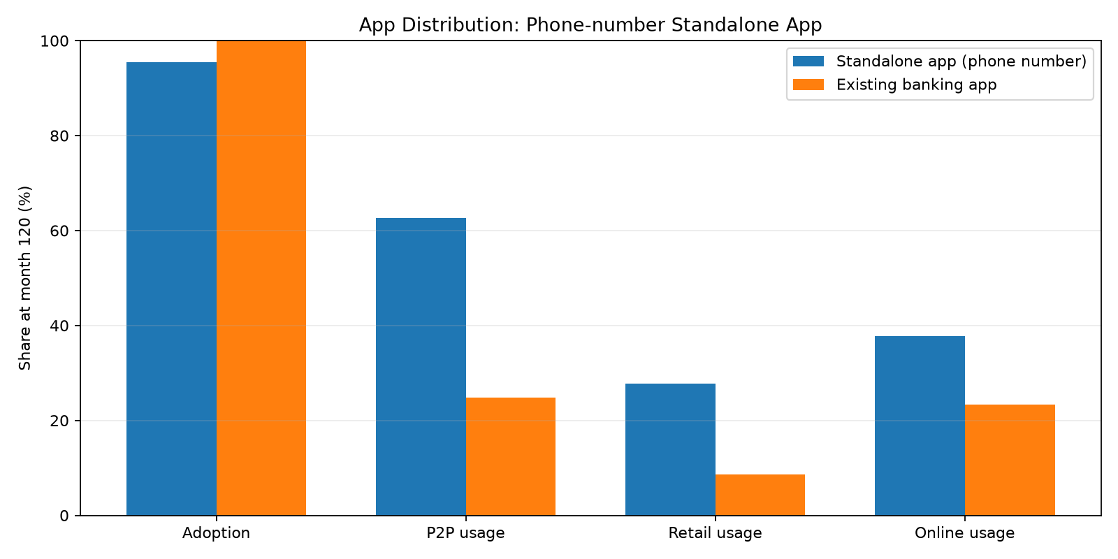
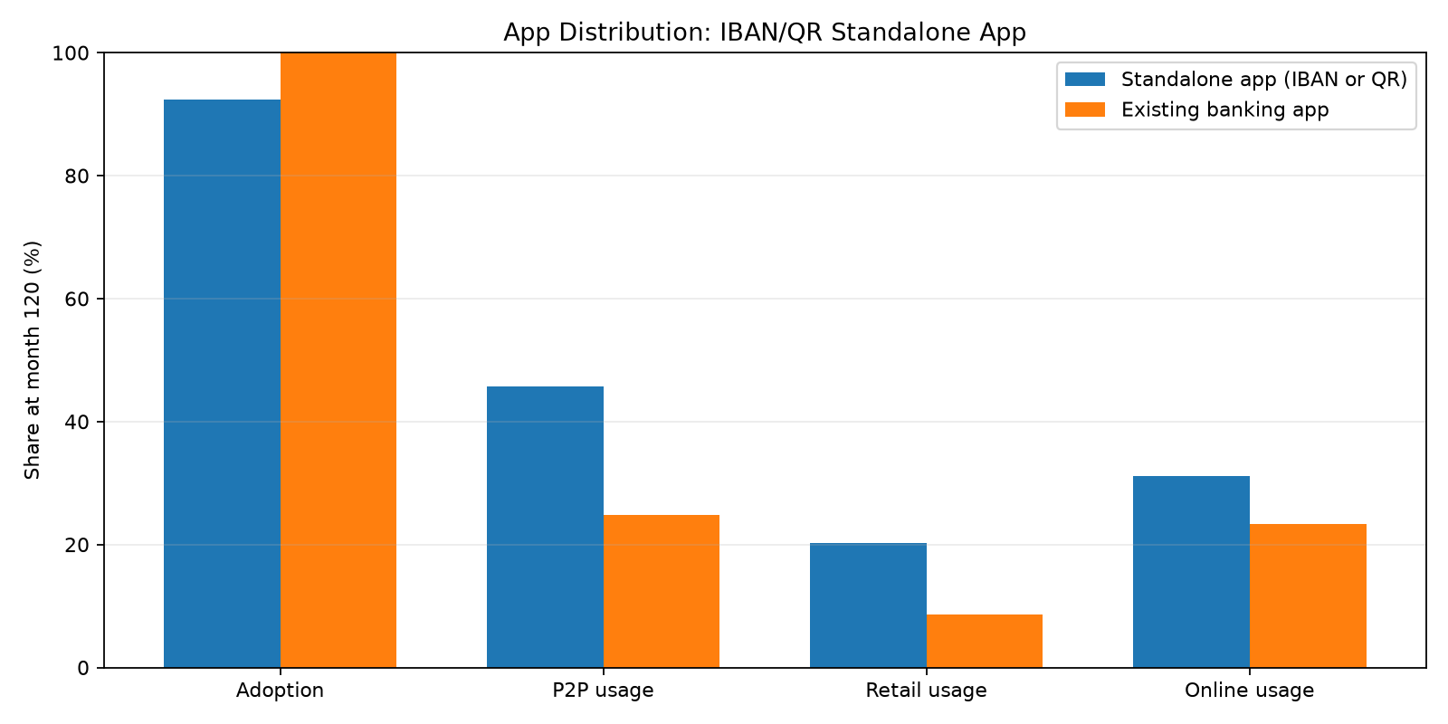
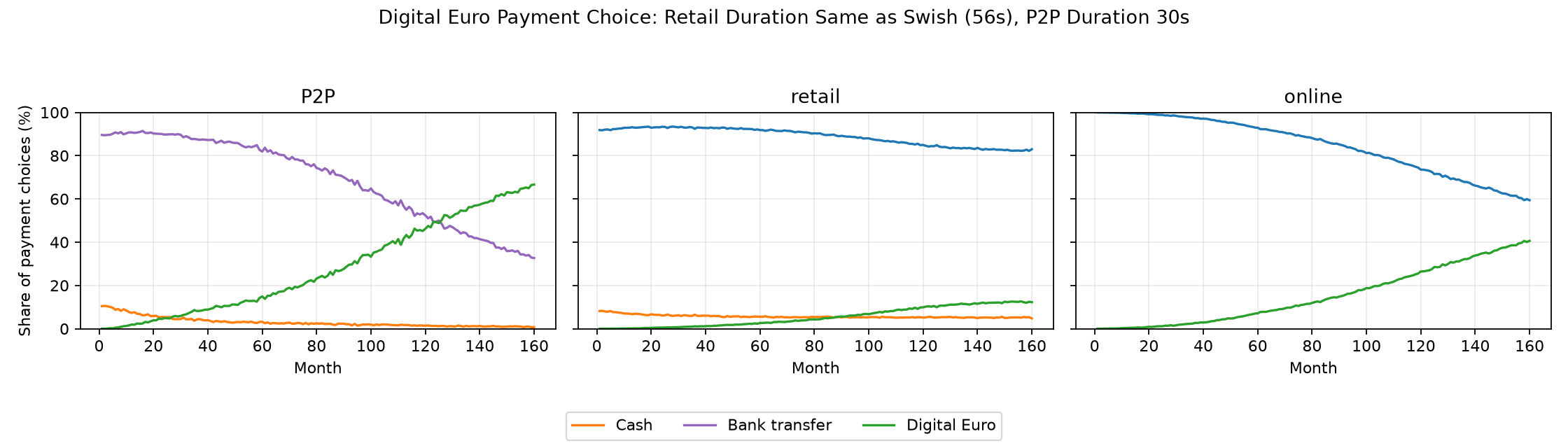
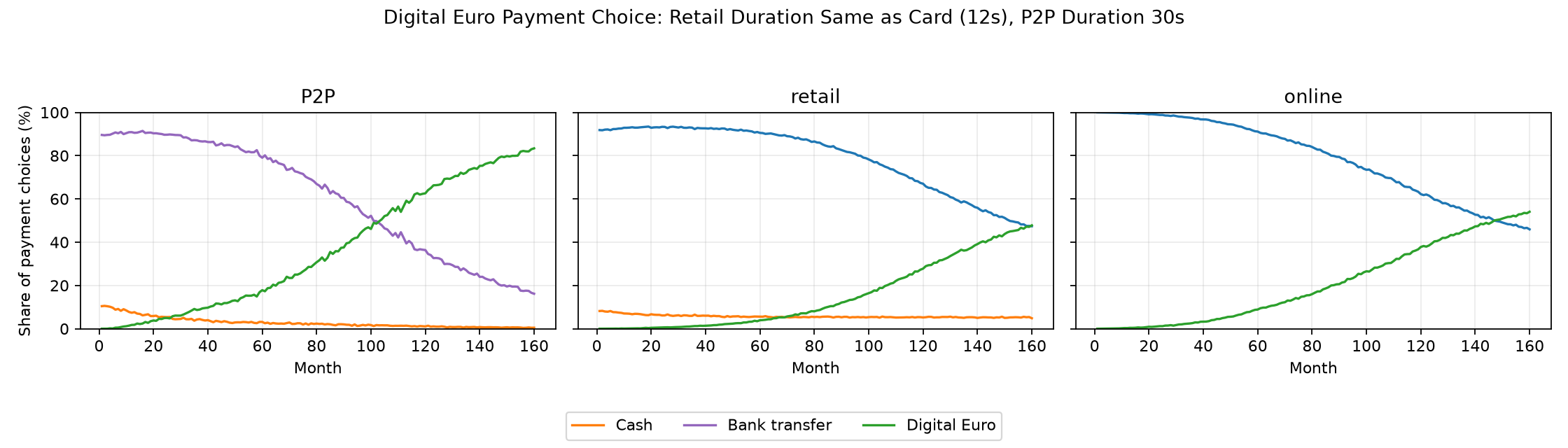
The two charts above use the 30-second P2P setting. The other retail charts are the 56-second P2P case with Swish-speed retail, the 56-second P2P case with card-speed retail, the 120-second P2P case with Swish-speed retail and the 120-second P2P case with card-speed retail.

More technical information and information on running the code is in the Github repository.